From Points to Flowy Curves
This project consists of two parts:
“Take a Spline for a Walk”
art project released on Bootloader
More about this project here>>
“From Points to Flowy Curves”
YouTube tutorial
The transcript of the video with few aditions and all the code examples>>
Introduction
Splines are a new set of functions in p5.js 2.0.
Before p5.js 2.0, you could have been using curve() and curveVertex() to create shapes and curves that slope gently. New set of functions replaces old curve, and introduces some features that will make creating contiunous shapes much easier. This document is partialy transcript of my video tutorial part of P5js Artist Series with few aditions and all the examples.
What is a spline?
In math, curves are described by using polynomial functions. There are many types, but in p5.js you’ll find two: Bézier curves and Catmull–Rom curves. Bézier curves let you define any shape imaginable, but they can also be a bit more complex to work with. On the other hand, Catmull–Rom curves are easier to grasp and quicker to build.
Generally, when we use term splines, we’re referring to a series of curves connected together into one continuous line. Instead of separate segments, they look as a single, flowing shape.
A simple way to picture this is like bending a cable smoothly around a set of pins. Each segment of the spline is defined by two points — beginning and ending — but also by the points just before and after. Those neighboring points influence how the curve bends as it passes through.
How to use spline()
In p5.js editor we will choose any version above 2.0, because these versions support new spline functions.
Let’s start with a simple example of storing positions of ten radom points in an array. We’ll do that in the setup().
Then in the draw() we can draw a polygon shape if we list all x and y positions for each array element in a vertex(x,y) function, enclosed between beginShape() and endShape().
Adding CLOSE as an argument to endShape(), it will also connect the last point to the first one, turning the line into a closed shape.
By simply replacing vertex() with splineVertex() we can turn the polygon into a smooth, continuous curve.
So with just one small change, we move from a low-poly shape to something much more fluid.
Note: if you need just one segment of the spline, you can use spline(x1,y1, x2,y2, x3,y3, x4, y4) without begin/endShape. (x1,x1) and (x4,y4) act as control points, and influence the curvature of the shape.
Spline properties
For each Catmull–Rom segment, the curve actually depends on four points. The inner points define where the line passes, while the outer ones influence how it bends.
splineProperty('ends', INCLUDE) is the default - before and after segments are included in the curve. You would use EXCLUDE to leave them out.
There’s also the question of how much the curve bends. That’s controlled by splineProperty('tightness', value).
You can think of it as adjusting how strongly the curve pulls between points. At 0, you get the default Catmull–Rom behavior. At 1, the curve straightens into lines.
This function also accepts higher and lower values, so let's check out how the curve behaves with other values. If we map horizontal mouse position (mouseX) to values between -2 and 2 we can see how this spline behaves when tighntess value changes.
Also, we can switch between INCLUDE and EXCLUDE values for the ends property when we use mouse vertical position (mouseY).
Math for shapes
In generative art, we’re often searching for balance between chaos and order.
So, instead of placing points completely at random, we can arrange them into different shapes using some trigonometry or math functions.
For placing points along a cricle we would use simple trigonometry.
For the angle between 0 and TWO_PI (TAU), we can calculate positions with these equations:
x = cos(angle)*radius

y = sin(angle)*radius
We can flatten a circle with this formula:
x = sin(cos(angle))*radius

y = sin(sin(angle))*radius
Form a four-pointed star:
x = cos(angle)5*radius

y = sin(angle)5*radius
A shape with few or many petals. By changing 6 to any other number will reflect in the change of the shape.
x = cos(6*angle)/6+cos(angle)

y = sin(6*angle)/6+sin(angle)
Or by adding a bit of randomness in the circle equations. For example, let’s place points around a circle but vary their distance from the center; each point gets a new position after reload.
Three animations and style examples
Step further would be to replace random() with noise(), and then we get smooth animation of an almost organic, blobby shape.
From here, we can explore a few variations. Let’s remove the decorations, and restyle the bob a bit. While we’re at it lets also separate recalculating noise positions from actual drawing of the shape.
Stop clearing the background and the previous frames stay visible on the canvas. And add a little bit of global movement…
If we draw the same blob twice, and make the top one with slightly thinner stroke weight, we can get an outline effect.
Adding a third copy can give us a simple shadow.
And one of my favorite tricks is stacking copies slightly offset and in darker shade until the form starts to feel dimensional. It’s not truly 3D, but it creates that illusion.
Final version of Rubber Bands
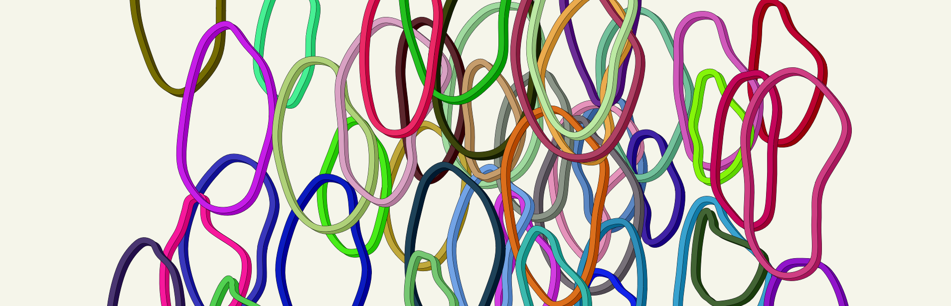
In the final step, I’ve converted the construction of “rubber bands” to a Class, and then generated many instances in the setup and also added a function for adding new ones on click. Each rubber band, has a different shape, movement and color.
Point on spline and tangent
If this got you interested in drawing with splines, there are two more really useful functions you can explore. What if you want to place something anywhere on the curve segment? Or have it just touch the curve, stay perpendicular to it, or keep a consistent distance as it moves along the curve?
That’s where splinePoint() and splineTangent() come in.
splinePoint() lets us find an exact position along a curve segment. We pass a value between 0 and 1 as last argument — where 0 is the start of the segment, and 1 is the end — and the function returns the coordinates of the point on the curve at that chosen position.
splineTangent() works in a similar way, but instead of position, it gives us the tangent at chosen position on a spline. Once we have that, we can calculate the angle, rotate it to get a normal, or position something around the curve.
In the next example I'm using both functions to position point on the curve, and to draw a tangent from that point.